
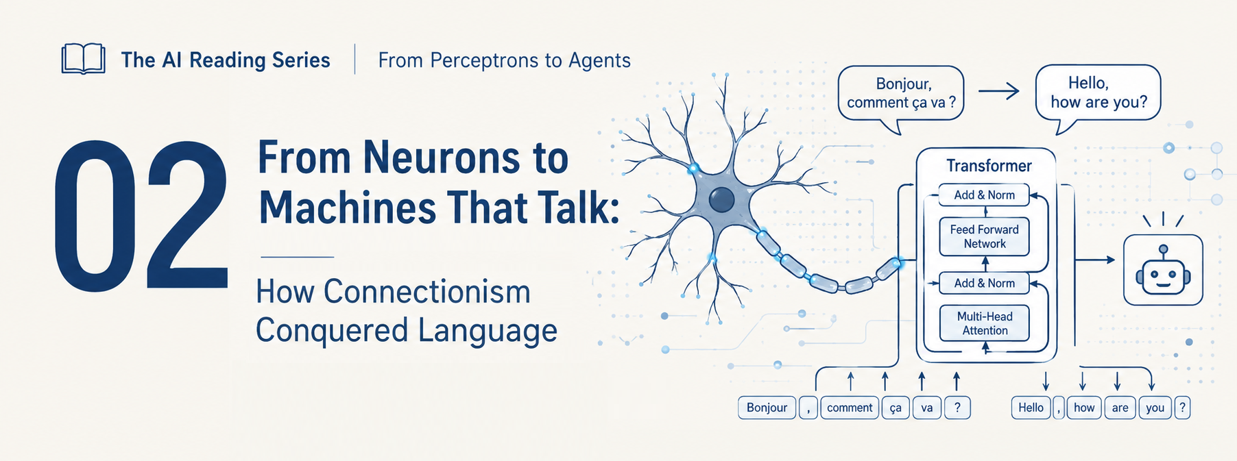
Part 2 of the AI reading series. Read this after Part 1: Where Machine Learning Came From.
The paper covered in the previous post of this series ends at the moment neural networks triumph: 2012, image recognition, ImageNet, the AlexNet “earthquake.” It gave us a precious reading grid — the world, the calculator, the horizon — and one central idea: connectionist machines won by emptying the calculator of all explicit rules, letting enormous masses of data shape the program themselves.
But Cardon and his colleagues talk mostly about images. The paper you are about to read next, “Attention Is All You Need“, is about language — machine translation, to be precise. And there is a world of difference between recognizing a rhinoceros in a photo and translating a sentence from French to English. This post tells the story of that road: how, between the mid-1980s and 2017, researchers adapted neural networks to the most “symbolic” problem there is — words, sentences, meaning — until they produced the architecture that now dominates all of artificial intelligence: the Transformer, the building block of Large Language Models (LLMs) such as ChatGPT, Claude, Gemini, and Qwen.
We will start simple and ramp up the technicality progressively. At the end you will find a timeline and a glossary: keep them at hand while reading Vaswani et al.
1. The problem images never posed: sequence
Let’s pick up where the previous paper left off. In 2012, a convolutional neural network (CNN) crushes the ImageNet competition. Why does convolution work so well on images? Because an image is a spatial object: a rhinoceros is still a rhinoceros whether it stands on the left or the right of the photo. The CNN exploits this property by sliding small filters across the image, like a magnifying glass sweeping over a photograph.
Language poses a different problem. A sentence is a sequence: a temporal, ordered object of variable length.
- “The dog bites the man” and “The man bites the dog” contain the same words, but order changes everything.
- The meaning of a word can depend on words that are far away: in “The key that I left on the kitchen table last night has disappeared,” the verb agrees with “the key,” a dozen words earlier. This is called a long-range dependency.
- A sentence can be 3 words or 300: the network must accept inputs of variable size.
Remember the formula from the previous post: for connectionists, the goal is to “put the world into a vector.” Two questions immediately arise, and the whole story that follows is a series of answers to them:
- How do you turn a word into a vector? (the representation problem)
- How do you process a variable-length sequence of vectors? (the architecture problem)
2. First answer: turning words into vectors
The word as a number (and why it is not enough)
The naive approach gives each dictionary word a number: “cat” = 4,812, “dog” = 1,953. Technically, one uses a so-called one-hot vector: a huge vector of zeros with a single 1 at the word’s position. The problem? In this representation, “cat” is no closer to “dog” than to “umbrella.” All resemblance between words is lost. It is a symbolic representation in the sense of the previous post: each word is a discrete symbol, identical to or different from another, with no internal structure.
Word2vec (2013): meaning as neighborhood
The solution was already hinted at in Cardon’s paper: word2vec (Mikolov et al., 2013). The idea rests on an old linguists’ intuition, summed up by John R. Firth in 1957: “You shall know a word by the company it keeps.” “Cat” and “dog” appear in similar contexts (“feed the ___”, “the ___ is sleeping”); they should therefore receive nearby vectors.
Word2vec trains a small neural network on a simple task: guess a word from its neighbors (or the reverse). The network is not the point; what you keep are the vectors learned along the way, called embeddings. Each word becomes a point in a space of a few hundred dimensions, and this space has astonishing properties:
- words that are close in meaning are close in distance;
- some directions of the space mean something: the famous computation king − man + woman ≈ queen actually works.
Now reread that sentence from Cardon’s paper: semantic proximity is not deduced from a symbolic categorization, but induced from statistical neighborhoods. This is exactly the symbolic-to-connectionist reversal, applied to the meaning of words. No linguist wrote a rule; meaning emerged from data. The first of our two problems — representing words — is solved.
But word2vec has a serious limitation: each word gets one single, fixed vector. Yet “bank” does not mean the same thing in “I called my bank” and “I sat on the river bank.” What we would need are contextual representations that change with the sentence. Keep this limitation in mind: the Transformer is, among other things, the machine that will blow it away.
3. Second answer: recurrent networks, a memory that reads word by word
The RNN: a loop over time (1986–1990)
There remained the second problem: processing a variable-length sequence. The historical answer is the recurrent neural network (RNN), popularized by Jeffrey Elman in 1990 and already present in the work of the PDP group of Rumelhart and Hinton (1986) — the same group as in Cardon’s paper.
The idea is elegant: the network reads the sequence one word at a time, left to right, and maintains a hidden state — a vector acting as working memory. At each word, the network combines what it reads with what it remembers, and updates its memory:
memory(t) = f( memory(t−1), word(t) )
Picture someone reading a sentence under their breath while keeping a mental summary they revise at every word. That is an RNN. The architecture naturally accepts sentences of any length: you simply loop for more or fewer steps.
The vanishing gradient problem
In practice, simple RNNs have a crippling flaw. Remember backpropagation: to learn, the error is propagated backwards through the network. In an RNN, “backwards” means back through time, across as many steps as there are words. At each step, the error signal is multiplied by coefficients; over a long sentence it gets multiplied dozens of times by numbers that are often smaller than 1… and it melts like snow in the sun. This is the famous vanishing gradient problem, identified notably by Sepp Hochreiter as early as 1991.
The concrete consequence: the network cannot learn long-range dependencies. By the time it reaches the verb “has disappeared,” it has “forgotten” the key at the beginning of the sentence.
The LSTM (1997): a memory with gates
The most celebrated solution arrives in 1997: the LSTM (Long Short-Term Memory), by Sepp Hochreiter and Jürgen Schmidhuber. The idea: equip the memory cell with learned gates — small mechanisms that decide, at each step, what to write into memory, what to forget, and what to read. A kind of whiteboard with a doorkeeper choosing what gets noted and what gets erased. Thanks to an internal “conveyor belt” where information circulates almost untouched, the gradient survives much longer.
LSTMs (and their simplified cousin, the GRU, 2014) would dominate natural language processing for twenty years. They are a perfect example of what Cardon’s paper calls the work on hyper-parameters and architecture: you do not dictate grammar rules to the network — you sculpt its structure so it can learn what it needs.
Around 2014–2015, boosted by GPUs and large corpora, LSTMs power the speech recognition in your phone and the first neural versions of Google Translate. Connectionism, victorious over images in 2012, is winning over language. But it is precisely by pushing LSTMs to their limits that the missing link will be discovered.
4. Translating: the seq2seq model and its bottleneck
Encoder–decoder (2014)
Machine translation is THE queen of tasks, because it demands everything: understanding one sequence and producing another, of a different length. In 2014, two teams (Sutskever, Vinyals and Le at Google; Cho and Bengio in Montreal) propose the seq2seq (sequence-to-sequence) architecture, made of two RNNs:
- an encoder reads the source sentence (“Le chat dort”) and compresses it into a single vector — a numerical summary of the whole sentence, sometimes called a “thought vector”;
- a decoder starts from this vector and generates the target sentence word by word (“The,” then “cat,” then “sleeps”), each produced word being fed back in to produce the next.
Note this word-by-word generation mechanism, each word conditioned on the previous ones: it is called auto-regressive, and it is exactly how ChatGPT or Claude write their answers today. This point from 2014 has never changed.
The bottleneck
But seq2seq has an obvious Achilles heel: the entire source sentence, whether 5 or 60 words long, must fit into a single fixed-size vector. It is like asking a translator to read a whole paragraph, close the book, then translate from memory without ever reopening it. On long sentences, quality collapses. Researchers call this the information bottleneck.
The solution will give its name to the paper you are about to read.
5. Attention: letting the network look wherever it wants
In 2014, Dzmitry Bahdanau, Kyunghyun Cho and Yoshua Bengio (him again — find him in the connectionist core of Cardon’s figure 2) publish an idea that changes everything: what if, instead of closing the book, the decoder could keep it open?
Concretely: the encoder no longer produces a single vector, but keeps one vector per word of the source sentence. Then, for every word it generates, the decoder computes a relevance score between what it is currently doing and each of the source words. These scores, turned into percentages (via a function called softmax), are used to build a weighted average of the source vectors: the decoder “focuses” on the words that are useful at that instant. To produce “sleeps,” it looks mostly at “dort.” This mechanism is called attention.
Three things to remember, because they directly prepare your reading of Vaswani et al.:
- Attention is learned, not programmed. Nobody wrote a French–English alignment rule: the network discovers by itself that “dort” explains “sleeps.” Once again, the inductive move described by Cardon — empty the calculator, let the world provide the structure.
- Attention is soft: it is not a binary choice but a weighting, therefore it is differentiable, therefore backprop applies to it.
- Attention creates shortcuts: every generated word is directly connected to every source word, without going through the fragile chain of recurrent memory. Long-range dependencies become connections… of distance 1.
Between 2015 and 2017, the “LSTM + attention” recipe becomes the world state of the art in translation (Google deploys it at the end of 2016). But an irritation grows among engineers, and it is a hardware one — remember the role of GPUs in Cardon’s story. An RNN reads a sentence word after word: computing word 50 must wait for word 49. Yet GPUs are massively parallel machines, built to perform millions of operations at the same time. Recurrence wastes the hardware and forbids training on truly gigantic corpora in reasonable time.
Hence a question asked ever more insistently in the labs: now that we have attention, what is recurrence still for?
6. “Attention Is All You Need”
The answer from eight Google researchers (Vaswani, Shazeer, Parmar, Uszkoreit, Jones, Gomez, Kaiser, Polosukhin) fits in their slightly provocative title: attention is all you need. Their architecture, the Transformer, purely and simply removes recurrence (and convolution). Here, as a preview, are the ideas you will meet in the paper — consider this section your reading map.
Self-attention
Until now, attention connected the decoder to the encoder (target to source). The Transformer’s stroke of genius is to apply it inside a single sentence: every word looks at every other word of its own sentence — including itself — to build its representation. In “The animal didn’t cross the street because it was tired,” the word “it” learns to attend to “the animal.” In one operation, each word enriches its meaning with its whole context.
Notice what this solves: a word’s vector is no longer fixed as in word2vec — it is contextual, recomputed for every sentence. “Bank” will not have the same representation at the counter and by the river.
Query, Key, Value: the library metaphor
The paper formalizes attention with three vectors per word, obtained through three learned transformations: a Query, a Key, and a Value. The classic image: in a library, you arrive with a question (your query), you compare it to the labels on the spines of the books (the keys), and you leave with the content of the relevant books (the values), in proportion to their relevance. Mathematically: dot products between Q and K → scores → softmax → weighted average of the V. That is equation (1) of the paper, the only truly indispensable one:
Attention(Q, K, V) = softmax(QKᵀ / √d) · V
The √d in the denominator is a mere numerical safeguard (keeping the scores from growing too large). Everything else in the paper is engineering around this formula.
Multi-head, position, and the full architecture
- Multi-head attention: rather than one attention, you run 8 (or 16, or 96…) in parallel, each with its own Q, K, V. Each “head” specializes — one tracks syntax, another coreference, and so on — without anyone asking it to. Emergent behavior, again.
- Positional encoding: removing recurrence has a cost — the network no longer knows in what order the words are! (Attention is a set computation, insensitive to order.) The fix: add to each embedding a small vector encoding its position, built from sines and cosines of varying frequencies. Do not drown in the formulas: just remember that we re-inject the order we lost.
- Stacking: one Transformer “block” = self-attention + a small classical network (feed-forward), with two training stabilizers (residual connections and normalization). These blocks are stacked: 6 in the 2017 paper, 96 and more in today’s LLMs. The original paper keeps the encoder–decoder structure inherited from seq2seq, since it targets translation.
- Parallelism: all words are processed at the same time. No more sequential waiting: the Transformer fits GPUs perfectly. This is the decisive argument — less training time, more data ingested. Reread Cardon: the connectionist victory has always been as much about hardware as about ideas.
7. From the Transformer to the LLM
The 2017 paper is about translation. How do we get to ChatGPT? Through an idea of disarming simplicity: next-word prediction.
Take a text, hide the next word, ask the model to guess it, correct it with backprop, repeat — trillions of times, over the whole web. No human labels are needed: the text is its own correction. This is called self-supervised learning. Think back to Cardon’s “horizon”: here, the horizon of the computation (the next word) is supplied by the world itself, for free, at unlimited scale. It is the ultimate cybernetic loop.
The key milestones:
- 2018 — GPT-1 (OpenAI): keep only the decoder of the Transformer, trained to predict the next word, then fine-tuned on specific tasks. BERT (Google) makes the opposite choice — keep only the encoder, trained to guess masked words — and crushes the comprehension benchmarks. The two descendants of the 2017 paper divide up the world.
- 2019 — GPT-2: same recipe, ×10 on size (1.5 billion parameters). Surprise: the model can summarize, translate, answer questions without having been trained to — simply because predicting the next word across the whole Internet forces it to learn a bit of everything.
- 2020 — GPT-3 and the scaling laws (Kaplan et al.): performance grows in a regular, predictable way with three ingredients — parameters, data, compute. The message: bigger is better, and nobody sees the ceiling yet. GPT-3 (175 billion parameters) reveals in-context learning: give it two examples inside the question (the prompt), and it picks up the pattern without any retraining.
- 2022 — ChatGPT and RLHF: a raw LLM completes text; it does not “answer.” It is aligned in two stages: fine-tuning on dialogues written by humans, then reinforcement learning from human feedback (RLHF) — annotators rank answers, the model learns to aim for the best-ranked ones. Note the historical irony: the horizon of the computation, expelled from symbolic rules, comes back through the door of human preferences.
- 2023–today: the era of open models (Meta’s Llama, Mistral, Alibaba’s Qwen), of multimodal models (text + image + sound), and of the Transformer’s extension to… image and video generation. Modern diffusion models (Stable Diffusion 3, Flux, Qwen-Image, Sora, Wan) have also replaced their old internal networks with Transformers (the so-called DiT, Diffusion Transformer, architecture). The 2017 architecture has become the universal architecture of connectionism.
One last thing, to close the loop with Cardon. The final table of his paper describes deep learning as: world = vectors of massive data, calculator = deep network, horizon = error optimization on an objective. The LLM is its most extreme culmination: the world is all the text ever written, the calculator is a Transformer with hundreds of billions of coefficients, and the horizon fits in three words — predict the next word. That capacities for reasoning, translation and dialogue emerge from such a poor objective is perhaps the most beautiful posthumous victory of the connectionist camp — and the philosophical question remains wide open, exactly where Cardon left it: what does a machine “understand” when its entire thought is, in Hinton’s phrase, “a big vector of neural activity”?
The paper is 11 dense pages. Reading advice:
- Read in this order: the abstract → the introduction (§1) → figure 1 (the architecture — keep it in view at all times) → §3.2 (attention, the heart of the paper) → the conclusion. The rest (§5–6, training details and translation results) can be skimmed.
- Do not get stuck on the math. Only one equation matters (Attention(Q,K,V), equation 1), and you already know its intuition: query → labels → weighted contents.
- Spot the words you now own: recurrent, sequential computation, long-range dependencies, parallelizable — you now know why they are there and what the paper is fighting against.
- A question to hold onto as you close the paper: why does removing recurrence make the addition of positional encoding mandatory?
Timeline
| Year | Event | Why it matters |
|---|---|---|
| 1943 | Formal neuron (McCulloch & Pitts) | The atom of connectionism |
| 1957 | Perceptron (Rosenblatt) | First learning machine |
| 1969 | Perceptrons (Minsky & Papert) | The “excommunication,” connectionist winter |
| 1986 | Backprop popularized (Rumelhart, Hinton, Williams) | Deep networks become trainable |
| 1990 | Elman’s RNN | The network that reads sequences |
| 1991/1997 | Vanishing gradient identified / LSTM (Hochreiter & Schmidhuber) | A memory that goes the distance |
| 2012 | AlexNet wins ImageNet | The “earthquake” — where the previous lecture ends |
| 2013 | word2vec (Mikolov) | Words become vectors of meaning |
| 2014 | seq2seq (Sutskever; Cho) | Encoder–decoder, auto-regressive generation |
| 2014–15 | Attention (Bahdanau, Cho, Bengio) | The decoder keeps the book open |
| 2016 | Google Translate goes neural | Connectionism conquers mainstream language |
| 2017 | “Attention Is All You Need” (Vaswani et al.) | The Transformer: attention alone, parallel compute |
| 2018 | GPT-1 (decoder) and BERT (encoder) | The two lineages of the Transformer |
| 2019 | GPT-2 | The “free” capabilities of next-word prediction |
| 2020 | GPT-3, scaling laws | Bigger = predictably better |
| 2022 | ChatGPT (RLHF) | The LLM becomes a conversational assistant |
| 2023 | Llama, Mistral, Qwen, DiT | Open models; the Transformer invades image/video diffusion |
Glossary
Attention — A learned mechanism that computes, for a given element, relevance weights over a set of other elements, then takes their weighted average. Enables direct connections between distant words.
Auto-regressive — Generation mode in which each new word is produced conditioned on all previous ones, one by one. This is how GPT, Claude and Qwen “write.”
Backpropagation — The algorithm (1986) that propagates the error from output to input to adjust the network’s weights.
BERT (2018) — Encoder-only model, trained to guess masked words; excellent at understanding text (classification, search).
Context window — The maximum number of tokens the model can consider at once. A major practical limit of LLMs.
Decoder — The half of the Transformer that generates the output sequence. GPT and most current LLMs are decoder-only.
Embedding — Representation of an object (word, image, molecule…) as a dense vector in a space where geometric proximity reflects similarity.
Encoder — The half of the Transformer that reads and represents the input sequence.
GRU / LSTM — Gated recurrent cells (1997 for the LSTM) that protect information over long stretches.
Hyper-parameters — Architecture and training choices set by humans (number of layers, heads, learning rate…), as opposed to learned parameters.
In-context learning — A model’s ability (from GPT-3 onwards) to pick up a task from a few examples placed directly in the prompt, without retraining.
LLM (Large Language Model) — A Transformer (usually decoder-only) with billions of parameters, trained by next-word prediction on immense corpora.
Long-range dependency — A grammatical or semantic link between words that are far apart in a sentence. Achilles heel of RNNs, strong point of attention.
Multi-head attention — Running several independent attentions (“heads”) in parallel, each free to specialize in one type of relation.
Parameters (weights) — The coefficients adjusted during learning. GPT-3: 175 billion. These are what you download when you fetch a model from Hugging Face.
Positional encoding — Vectors added to the embeddings to re-inject word order, which attention alone ignores.
Prompt — The input text given to the LLM; since GPT-3, you “program” the model in natural language through the prompt.
Query / Key / Value (Q, K, V) — The three learned projections of each word used in the attention computation: the question asked, the label compared, the content retrieved.
RLHF — Reinforcement Learning from Human Feedback: aligning an LLM with human preferences via reinforcement (the basis of ChatGPT, 2022).
RNN (recurrent neural network) — A network that processes a sequence step by step while maintaining a hidden state (memory). Dominant in NLP from 1990 to 2017.
Scaling laws — Empirical relations (2020) showing that LLM performance improves predictably with model size, data and compute.
Self-supervised learning — Learning without human labels: the data provides its own target (e.g., the next word of a text).
Seq2seq — The encoder–decoder architecture (2014) turning one sequence into another; the framework of neural translation and the direct ancestor of the Transformer.
Softmax — The function that converts a list of scores into a probability distribution (percentages summing to 100%). Used inside attention and to pick the next word — it is on this function that the temperature parameter operates.
Token — The elementary unit of text a model manipulates (often a word fragment, ~¾ of a word on average).
Transformer (2017) — Architecture based solely on attention (no recurrence, no convolution), massively parallelizable; the foundation of all LLMs and, by now, of diffusion models (DiT).
Word2vec (2013) — A method producing static word embeddings from their contexts of occurrence; the ancestor of the Transformer’s contextual representations.
Watch After Reading
- 3Blue1Brown — the Transformer chapters of the Deep Learning series: “But what is a GPT?” then “Attention in transformers, step-by-step.” The finest visualization of equation (1) in existence.
- “Let’s build GPT: from scratch, in code, spelled out” — Andrej Karpathy (~2 h): building a GPT by following the paper, from tokenization to multi-head attention. Watch it with the code open.
Table of contents

Leave A Comment