Highlights
- Easy Python Setup: Learn how to install Python using Anaconda and configure a full environment for spatial analysis in just a few steps.
- Spatial Data Ready: Install essential libraries like GeoPandas, Pyogrio, and Contextily to start working with geospatial datasets immediately.
- Work in Jupyter:Use Jupyter Notebooks to write, visualize, and run spatial analysis code directly — perfect for beginners and researchers alike.
In this guide you’ll find clear instructions on setting up Python with Anaconda for spatial analysis. Then, we’ll cover installing Python alongside Anaconda and adding essential dependencies like GeoPandas via the Anaconda Prompt. Lastly, we’ll explore using the Jupyter Notebook for practical application. By the end, you’ll be ready to start your journey in Python-based spatial analysis, AI, and machine learning.
1. Install Python with Anaconda
Anaconda is a powerful tool for managing Python environments. Indeed, Anaconda simplifies package management through its integrated package manager, conda. In addition, it comes bundled with a set of pre-installed libraries commonly used in data science and spatial analysis, such as NumPy, Pandas or Matplotlib. Therefore, this eliminates the need for manual installation and ensures immediate access to these libraries. Anaconda is also cross-platform compatible (available for Windows, macOS, and Linux) thus providing consistent Python environments across different operating systems. Furthermore, it seamlessly integrates with popular development environments like Jupyter Notebook, known amongst other things for its user-friendly interface. Visit the Anaconda website and download the Anaconda distribution related to your operating system (Windows, macOS, or Linux). Once Anaconda is installed, you’ll have access to the Anaconda Navigator, Anaconda Prompt, and other useful tools for managing Python environments.
2. Install Additional Dependencies on Python using Anaconda Prompt
Even if the Python distribution installed by Anaconda comes with numerous pre-installed libraries, additional dependencies will be required to enable performing advanced manipulations, and this is especially true for manipulating spatial data. So, let’s install the following three dependencies to manipulate spatial data : GeoPandas : allow spatial operations on geometric types ; Pyogrio : interoperability between spatial data formats and Contextily : retrieve tile maps from the internet.
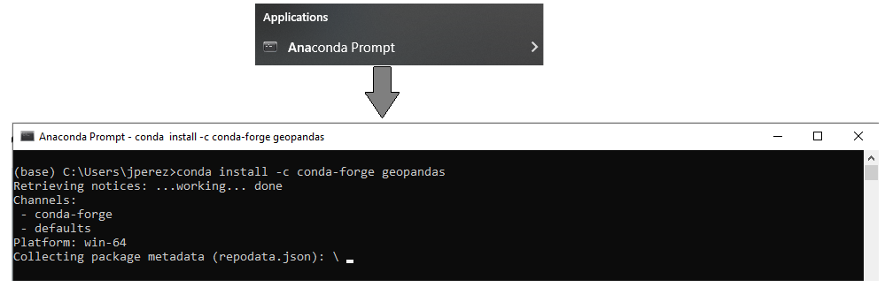
Then, on Windows, click on the Start Menu and type “Anaconda Prompt” in the search bar and open it. This will open a new command prompt window with Anaconda enabled. Within the command prompt, run the following commands one by one to install the aforementioned dependencies.
conda install -c conda-forge geopandas
conda install -c conda-forge pyogrio
conda install -c conda-forge contextily
If you’ve previously installed the libraries, executing these lines will not only update the libraries themselves but also their dependencies. Additionally, any other dependencies not encompassed within the Anaconda distribution of Python can be installed using the same commands. For instance, for machine learning purposes, you can install ‘XGBoost’ (eXtreme Gradient Boosting) using these lines as well.
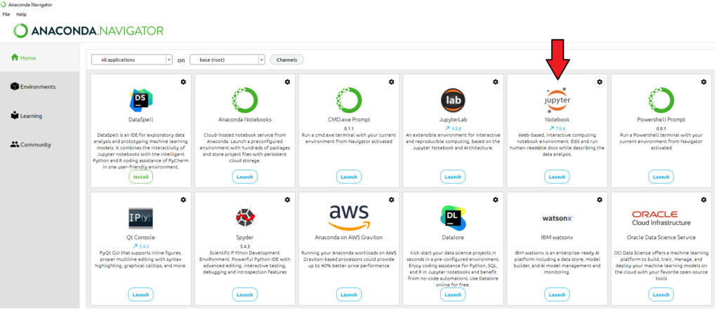
Now that you’ve installed Python and the required dependencies, you can open the Anaconda Navigator and launch the Jupyter Notebook from the Home tab, as follows:
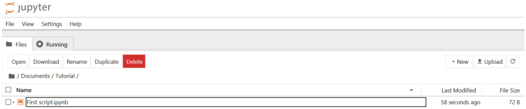
Jupyter Notebook is an open-source web application that allows users to create and share documents containing live code, visualizations, and narrative text. Upon launching the notebook, you’ll be directed to the Jupyter Notebook explorer in your default web browser, where you can create folders and new notebooks with a simple right-click action, as demonstrated below.
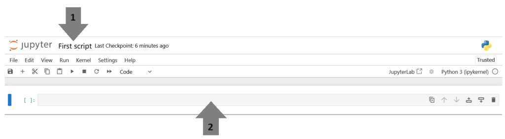
Afterward, you can rename your notebook (indicated by arrow 1 below). In a notebook, users can compose and execute code in segmented blocks. The figure below illustrates one such block (indicated by arrow 2 below).
4. Set a Working Directory and Load Data from Jupyter
Your notebook is automatically linked to the files within the folders where it resides. Let’s add some data to this folder and import it into the notebook (or Python environment). Begin by downloading the dataset provided below. This dataset comprises a GeoPackage file containing two building layers corresponding to two small cities in Italy: Grosseto and Sinalunga. For further insight related the GeoPackage format, you can refer to this post. Then, once you have downloaded, place it in the same directory as your notebook.
Then, you can run the code below to import a layer in Python using GeoPandas. In this example, we are importing a layer of building related to the italian city of Grosseto.
import geopandas as gpd
Grosseto = gpd.read_file("Italian_cities.gpkg", layer = "Grosseto")
Finally, you can run the code below to plot the building layer with a basemap from OSM using contextily.
import matplotlib.pyplot as plt
import contextily as ctx

# Plot the Grosseto layer
fig, ax = plt.subplots(figsize=(10, 10))
Grosseto.plot(ax=ax, alpha=0.5)

# Add basemap using Contextily
ctx.add_basemap(ax, crs=Grosseto.crs, source=ctx.providers.CartoDB.Voyager)
# Set title and show plot
plt.title("Grosseto with Basemap")
plt.show()
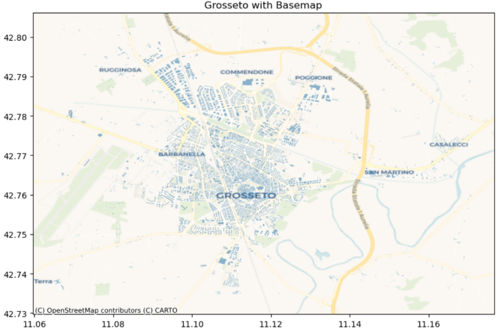
The map above was generated using the Python code provided — demonstrating how to overlay geospatial data with a custom basemap using contextily. Fell free to provide feedbacks on our blog posts by contacting us.
Table of contents

Leave A Comment