Highlights

• Setting Up Environment: Readers are guided through setting up a specific environment in Anaconda to control QGIS from the Jupyter Notebook
• Initializing QGIS in Python: The tutorial illustrates how to initialize QGIS within a Python script to ensure access to QGIS functionalities
• Running QGIS Algorithms from Python: A simple algorithm, “dissolve,” is executed as an example

QGIS, a leading open-source Geographic Information System (GIS), provides an interesting suite of tools for geospatial analysis. Have you ever wondered about controlling QGIS with a Python script ? About calling a specific tool within QGIS from Python? This capability can be useful to integrate processing already available in QGIS within a script of your own without opening the QGIS software directly. In this blog post, we’ll explore how to call QGIS from a Python script in the Jupyter Notebook. Let’s dive in.

1. Set Up a Specific Environnement for controlling QGIS with Python

If you’re new to Python or Jupyter Notebook, check out our introductory guide to set up a Python environnement using Anaconda. In this tutorial, we assume that you are using the Anaconda distribution of Python. The first step is to open your Anaconda prompt windows and create a Conda environment that includes both QGIS and Jupyter Notebook. On Windows, click on the Start Menu and type “Anaconda Prompt” in the search bar and open it. Within the command prompt, run the line below:

conda create -n qgis_jupyter qgis notebook

Now, you can activate the newly created Conda environment using the following command, also in the Anaconda prompt windows. Once you activate the qgis_jupyter environment, you’ll have access to QGIS and Jupyter Notebook within the same environment, allowing you to use QGIS functionality directly from your Jupyter Notebooks. If you have an issue with the code above, then run this conda install -c conda-forge qgis line of code.

conda activate qgis_jupyter

And finally, open a Jupiter Notebook within the environnement you just activated

jupyter notebook

2. Get your Environnement ready for controlling QGIS with Python and Import Test Data

Now that your notebook is open, you can run the code snippet below to set up the interaction with QGIS. Note that even if you don’t need to open the QGIS standalone, you need to have QGIS installed on your machine to interact with it. That’s why we need to specify in the code below the installation directory path of QGIS and initialize it. This ensures that the Python interpreter can locate the necessary QGIS libraries. Additionally, the script initializes the next processing algorithms that will be performed.

from qgis.core import QgsApplication, QgsProcessingFeedback
import processing
import sys

# Initialize QGIS Application
qgis_path = "C:/Program Files/QGIS 3.x/apps/qgis"
sys.path.append(qgis_path)
QgsApplication.setPrefixPath(qgis_path, True)
qgs = QgsApplication([], False)
qgs.initQgis()

# Add processing algorithms to registry
from processing.core.Processing import Processing
Processing.initialize()

Let’s work on Grosseto, one of the Italian city available in a layer within the following GeoPackage.

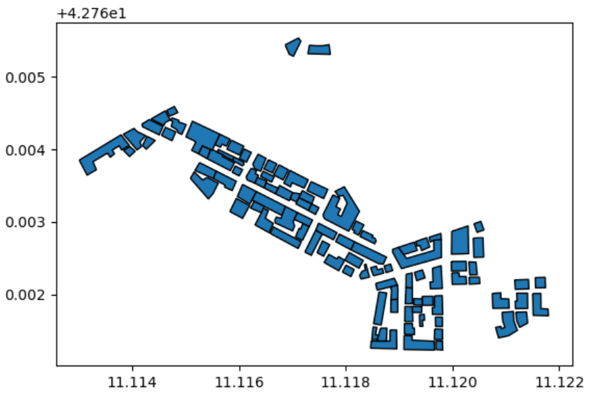
The layer contains the building footprints of Grosseto. Provided you put the GeoPackage in the folder where your notebook is located, you can already import and plot the layer, as shown below. For this example, we are working on a subset of 100 buildings.

import geopandas as gpd

# Read the layer "Grosseto" from the GeoPackage "Italian_cities.gpkg"
Grosseto = gpd.read_file("Italian_cities.gpkg", layer = "Grosseto")

# Subset 100 features (index 1500 to 1600)
Subset_Grosseto = Grosseto[1500:1600]

# Plot the subset with black borders
Subset_Grosseto.plot(edgecolor='black')

3. Calling a Single Algorithm : Dissolve

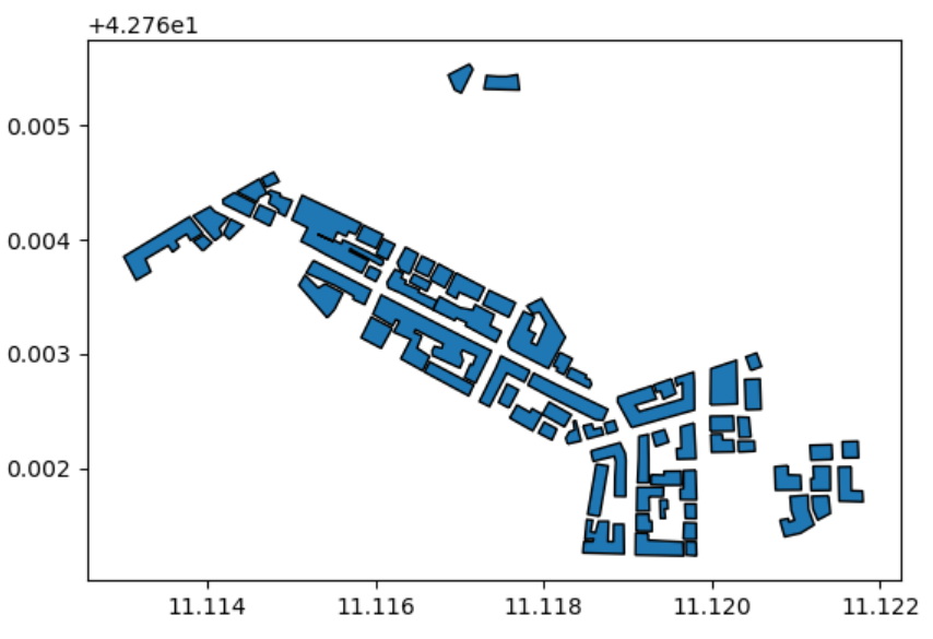
Now, let’s execute a straightforward algorithm, such as “dissolve,” by invoking the QGIS tool directly within the notebook and visualize the outcome to verify its success. Ensure to specify the location of the Geopackage in the code, along with defining the input and output layers. Subsequently, call the algorithm using the native:dissolve identifier, and adjust its parameters as necessary. The result, named Dissolved_Subset_Grosseto is saved as a new layer in the GeoPackage and ploted in the notebook.

# Define the path to the GeoPackage
gpkg = "C:\\Users\\...\\Italian_cities.gpkg"
# Define the input layer name
input_layer = "Subset_Grosseto"
# Define the output layer name
output_layer = "Dissolved_Subset_Grosseto"

# Run the dissolve algorithm
processing.run("native:dissolve", 
{'INPUT':f"{gpkg}|layername={input_layer}",
'FIELD':[],
'SEPARATE_DISJOINT':False,
'OUTPUT':f'ogr:dbname=\'{gpkg}\' table="{output_layer}" (geom)'})

# Read the layer "Grosseto" from the GeoPackage "Italian_cities.gpkg"
Dissolved_Subset_Grosseto = gpd.read_file("Italian_cities.gpkg", layer = "Dissolved_Subset_Grosseto")

# Plot the subset with black borders
Dissolved_Subset_Grosseto.plot(edgecolor='black')

As you can see below the buildings have been perfectly dissolved using the native QGIS algorithm.

4. Iterate a Single Algorithm with Different Parameters

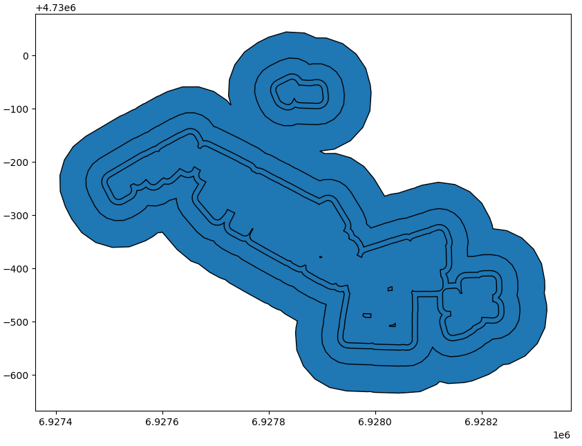
This code snippet below demonstrates a workflow in Python using the buffer QGIS algorithm. First, we reproject the input layer to a Cartesian Coordinate Reference System (CRS) suitable suitable for the buffer function. Subsequently, the script iterates through a series of distances, executing the buffer algorithm four times with varying distances (10, 20, 50, and 100 meters). Each buffer operation generates a new layer with the GeoPackage.

# Use a cartesian CRS for north Italy
Dissolved_Grosseto_Subset = Dissolved_Grosseto_Subset.to_crs(6875)
# Overwrite the layer with new CRS
Dissolved_Grosseto_Subset.to_file("Italian_cities.gpkg", layer="Dissolved_Grosseto_Subset", driver="GPKG")

# Define the input layer name
input_layer = "Dissolved_Grosseto_Subset"

# Iterate through buffer distances
for buffer_distance in [10, 20, 50, 100]:
    # Define the output layer name
    output_layer = f"Buffered_{buffer_distance}m"
    
    # Run the buffer algorithm 4 times with 10, 20, 50 and 100 meters
    processing.run("native:buffer", 
                   {'INPUT':f"{gpkg}|layername={input_layer}",
                    'DISTANCE': buffer_distance,
                    'SEGMENTS': 5,
                    'END_CAP_STYLE': 0,
                    'JOIN_STYLE': 0,
                    'MITER_LIMIT': 2,
                    'DISSOLVE': False,
                    'OUTPUT':f'ogr:dbname=\'{gpkg}\' table="{output_layer}" (geom)'})

Let’s map the different buffers. The code below import the layers we just created with a loop, and plot them in reverse order in order to visualize the overlap using Matplotlib.

buffer_distances = [10, 20, 50, 100]
buffer_layers = {}

for distance in buffer_distances:
    layer_name = f"Buffered_{distance}m"
    buffer_layers[f"Grosseto_Subset_Dissolved_Buffered_{distance}m"] = gpd.read_file("Italian_cities.gpkg", layer=layer_name)

# Create a Matplotlib axis
fig, ax = plt.subplots(figsize=(10, 8))

# Reverse the order of the layers
for layer_name, layer_data in reversed(buffer_layers.items()):
    layer_data.plot(ax=ax, edgecolor='black')

Feel free to engage with this post by commenting, asking questions, or providing feedback.