Highlights
- Run GeoPandas entirely in the cloud using Google Drive and Google Colab — no local setup required.
- Create and analyze a polygon around Paris with simple spatial operations like buffering.
- Save results back to Google Drive, completing your first cloud-based geospatial workflow.
Working with geospatial data has never been easier thanks to GeoPandas on Google Colab. This powerful combination lets you run Python scripts entirely in the cloud — no installation or setup required. In this tutorial, you’ll learn how to create, manipulate, and save geographic data using GeoPandas and Google Drive, all within a Colab notebook. We’ll build a simple polygon around Paris, apply a spatial buffer, and save the results directly to your Drive. By the end, you’ll have a lightweight, fully cloud-based workflow for reproducible geospatial analysis.
1. Setting Up Your Cloud Workspace
Before starting, open your Google Drive and create a new folder, for example named geospatial_colab_project. This folder will serve as your project directory, where you’ll store your notebooks, datasets, and outputs.
Once the folder is ready, go to Google Colab, create a new notebook, and connect it to your Drive. Colab allows you to run Python code on Google’s servers while accessing your Drive files as if they were local. This integration makes it ideal for lightweight, cloud-based geospatial processing.
You can connect your Drive with the following code that you will first add in a new code block (+ Code) and then Run by clicking on the play button.
from google.colab import drive

# Mount Google Drive
drive.mount('/content/drive')

# Set your working directory
import os
project_folder = '/content/drive/MyDrive/geospatial_colab_project'
os.chdir(project_folder)

print("Current working directory:", os.getcwd())
After executing the cell, Colab will prompt you to authorize access to your Google Drive. Once mounted, you’ll see a folder named MyDrive appear in the Colab file browser. All files you create or modify inside this folder will automatically sync to your Drive.

If everything went smoothly, the following line will be printed:
Current working directory: /content/drive/MyDrive/geospatial_colab_project
2. Installing and Importing GeoPandas
GeoPandas extends the popular Pandas library to handle geometric data such as points, lines, and polygons. For official documentation, visit GeoPandas.org. Install it directly in Colab:
!pip install geopandas shapely fiona pyproj
Then, import the necessary libraries:
import geopandas as gpd
from shapely.geometry import Polygon
3. Creating a Simple Polygon Around Paris
Let’s create a basic polygon — a simple rectangle surrounding Paris — directly from scratch using GeoPandas and Shapely.
# Define coordinates (longitude, latitude)
paris_bounds = [
    (2.20, 48.80),  # Southwest corner
    (2.20, 48.90),  # Northwest
    (2.45, 48.90),  # Northeast
    (2.45, 48.80),  # Southeast
    (2.20, 48.80)   # Close the polygon
]

# Create a Shapely Polygon
polygon = Polygon(paris_bounds)

# ✅ Create a GeoDataFrame properly
gdf = gpd.GeoDataFrame(, crs="EPSG:4326")

# Display the GeoDataFrame
gdf
4. Performing a Simple Geospatial Operation (Buffer)
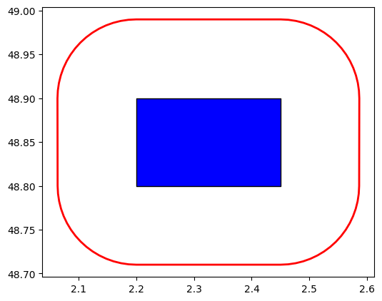
Now that you have your polygon, let’s perform a basic spatial operation — creating a 10 km buffer around Paris. This buffer will expand the polygon outward by 10,000 meters.
# Convert to a projected coordinate system for accurate distance (meters)
gdf_projected = gdf.to_crs(epsg=2154)  # Lambert-93 for France

# Create a 10 km buffer
gdf_buffer = gdf_projected.buffer(10000)

# Convert back to WGS84 for visualization
gdf_buffer = gpd.GeoDataFrame(geometry=gdf_buffer, crs="EPSG:2154").to_crs(epsg=4326)

# Plot both
ax = gdf.plot(color='blue', edgecolor='black', figsize=(6, 6))
gdf_buffer.plot(ax=ax, color='none', edgecolor='red', linewidth=2)

5. Saving the File Back to Google Drive
Once your data is processed, saving it back to Google Drive is straightforward. GeoPandas supports many file formats such as GeoJSON, Shapefile, and GeoPackage.
# Save as GeoJSON
output_path = os.path.join(project_folder, 'paris_buffer.geojson')
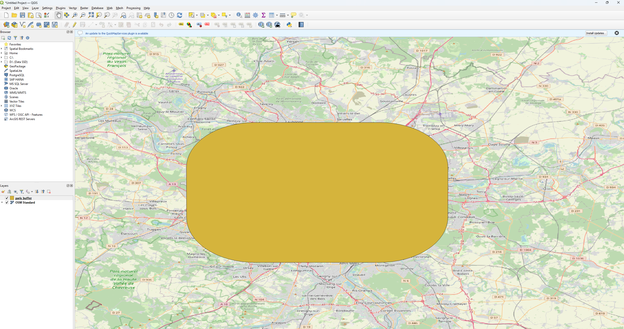
gdf_buffer.to_file(output_path, driver='GeoJSON')

With just a few lines of Python, you’ve connected Google Drive to Colab, created and visualized a polygon around Paris, applied a spatial buffer, and saved your results back to the cloud. This simple workflow demonstrates the power and accessibility of cloud-based geospatial computing — ideal for collaboration, education, and rapid prototyping without the need for heavy local setups.
6. Alternative Cloud-Based Geospatial Combos
While Google Drive + Google Colab is a convenient and free solution for quick experiments, other combinations can be equally effective depending on your workflow:
| Combo |
Description
|
|---|---|
| GitHub + Kaggle Notebooks | Store your data and notebooks on GitHub and run them on Kaggle’s cloud environment, which offers free GPUs and persistent datasets. |
| Dropbox + Colab | Similar to Drive integration, Dropbox can be mounted via API to provide additional storage flexibility. |
| AWS S3 + SageMaker Studio Lab | For more advanced workflows, S3 provides scalable data storage with SageMaker’s free-tier notebooks. |
| Google Earth Engine + Colab | The best option for satellite or raster data processing, with integrated access to massive Earth observation datasets. |
Don’t hesitate to comment and provide feedbacks by engaging with this post.
Table of contents


Leave A Comment