Highlights

• Data Preparation: Point data preparation using the Python library GeoPandas
• Calculating NND and generating CSR distribution: Nearest Neighbor Distance and generation of random points for comparison
• Interpreting Results: Comparison of observed NND values with CSR, indicating clustering, dispersion, or randomness
• Comparative Analysis: Comparative analysis example using two cities in Italy : Grosseto and Sinalunga

1. Complete Spatial Randomness : Theoretical Recap

CSR, or Complete Spatial Randomness, is a theoretical model used in spatial statistics to describe a random distribution of points in space. Essentially, in a CSR process, points are distributed randomly across the study area, with no clustering or spatial patterns. Each point is independent of the others and has an equal chance of occurring at any location within the study area.

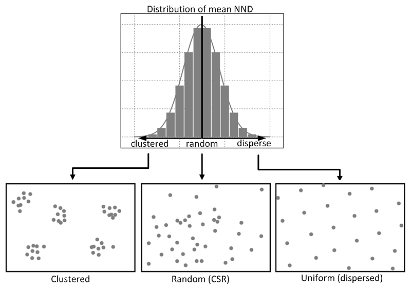
When comparing observed spatial patterns to CSR, it is important to note that if the observed pattern exhibits a mean nearest neighbor distance that is significantly smaller than the mean nearest neighbor distance of a random distribution (CSR), it suggests clustering. In other words, this means that points in the observed pattern are closer to each other on average than would be expected under a random process. Conversely, if the mean nearest neighbor distance of the observed pattern is significantly larger than that of a random distribution, it suggests dispersion. Consequently, this indicates that points in the observed pattern are farther apart on average than would be expected under a random process.

Figure 1 : Interpretation of Patterns from mean NND score (Source : Yuan et al., 2020)

Calculating Nearest Neighbor Distance (NND) and comparing it with CSR can be useful in various fields where spatial patterns play a crucial role, such as ecology (distribution of species) or urban planning. Let’s see together how to calculate a nearest neighbor distance from a given point pattern and compare it to a random distribution (CSR).

2. Spatial patterns of points : calculation of Nearest Neighbor Distance (NND) and comparison with CSR

2.1 Spatial patterns of points : Sample data

To perform this analysis, we will use two building layers. You can obtain OSM building data from various locations worldwide using the Overpass Turbo tool. The sample data used in this demonstration consists of two OSM building layers compiled into a Geopackage file.

This sample data pertains specifically to the Italian cities of Grosseto and Sinalunga, each containing approximately 7500 buildings.

import geopandas as gpd
import numpy as np
from scipy.spatial.distance import cdist
import matplotlib.pyplot as plt

# Read the layers for the two Italian cities
gdf_1 = gpd.read_file("Italian_cities.gpkg", layer = "Grosseto")
gdf_1 = gdf_1.to_crs(epsg=6875)
gdf_2 = gpd.read_file("Italian_cities.gpkg", layer = "Sinalunga")
gdf_2 = gdf_2.to_crs(epsg=6875)

The provided code imports necessary libraries and extracts each layer from the GeoPackage. For detailed guidance on configuring your Python environment and managing libraries, you can consult this post. Additionally, if you seek information on GeoPackage usage and layer importation into Python, you can refer to this post.

# Create a figure with two subplots
fig, axs = plt.subplots(1, 2, figsize=(20, 10))

# Plot gdf_1 in the first subplot
gdf_1.plot(ax=axs[0], color='blue', edgecolor='black')
axs[0].set_title("Map View of Grosseto")
axs[0].set_xlabel("Longitude")
axs[0].set_ylabel("Latitude")

# Plot gdf_2 in the second subplot
gdf_2.plot(ax=axs[1], color='red', edgecolor='black')
axs[1].set_title("Map View of Sinalunga")
axs[1].set_xlabel("Longitude")
axs[1].set_ylabel("Latitude")

# Adjust layout
plt.tight_layout()

# Display the plot
plt.show()

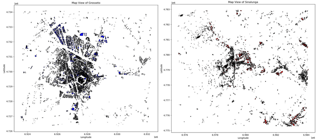
This code snippet creates a figure with two subplots. Specifically, in the first subplot, the map view of Grosseto is plotted, while Sinalunga is shown in the second plot. At first glance, buildings in both maps look clustered. However, it is difficult to visually assess which pattern is more clustered or dispersed than the other.

2.2 Generating a Distribution of Random Points

# Calculate the centroids of gdf_1
gdf_1_points = gdf_1.centroid
points_geom = gpd.GeoDataFrame(geometry=gdf_1_points)
# Extract coordinates from the centroids
coordinates = np.array([[points.coords[0][0], points.coords[0][1]] for points in points_geom.geometry])

# Calculate the bounding box of the GeoDataFrame
min_x, min_y, max_x, max_y = gdf_1.total_bounds
np.random.seed(123)  # Set seed for reproducibility

# Generate random points within the bounding box
random_points_x = np.random.uniform(min_x, max_x, 1000)
random_points_y = np.random.uniform(min_y, max_y, 1000)
# Create a GeoDataFrame from the random points
random_points_geom = gpd.GeoDataFrame(geometry=gpd.points_from_xy(random_points_x, random_points_y))

# Extract coordinates of the random points
coordinates_random = np.array([[point.x, point.y] for point in random_points_geom.geometry])

# Plot the random points
ax = random_points_geom.plot(markersize=1)
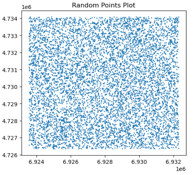
ax.set_title('Random Points Plot')
plt.show()

This code snippet demonstrates the process of generating random points within the bounding box of a given GeoDataFrame, which contains geographical data. To begin with, the centroids of the GeoDataFrame are calculated to determine the central points of each building, thus transforming the buildings into spatial patterns of points. Next, the total bounds of the GeoDataFrame are computed to define the bounding box, which encompasses all geometries. Subsequently, using the minimum and maximum coordinates of the bounding box, random points are generated uniformly within this spatial extent. After that, these random points are then organized into a GeoDataFrame for further analysis. Overall, this approach is commonly used in spatial analysis and simulation studies to simulate spatial processes or to create synthetic datasets for testing algorithms and methods.

# Function to calculate nearest neighbor distances
def nearest_neighbor_distances(points):
    # Calculate pairwise distances between points
    distances = cdist(points, points)
    np.fill_diagonal(distances, np.inf)  # Exclude distance to itself
    # Calculate nearest neighbor distances
    nearest_distances = np.min(distances, axis=1)
    return nearest_distances

# SD on the nearest neighbor distances
def nearest_neighbor_sd(points):
    # Calculate nearest neighbor distances
    nearest_distances = nearest_neighbor_distances(points)
    # Calculate standard deviation of nearest neighbor distances
    sd = np.std(nearest_distances)
    return sd

The nearest_neighbor_distances function calculates the nearest neighbor distances for a given set of points in a two-dimensional space. Specifically, it computes the pairwise distances between all points using the cdist function from SciPy’s spatial module. After that, by filling the diagonal of the distance matrix with infinity, it excludes distances to the points themselves. Consequently, it finds the minimum distance for each point, representing its nearest neighbor distance. Finally, the function returns an array containing the nearest neighbor distance for each point. This array is then used by the nearest_neighbor_sd function, which computes the standard deviation of nearest neighbor distances for a set of points.

3. Results and Interpretation of NDD and CSR results for spatial patterns of points

3.1 Assess clustering or dispersion

mean_observed_nn = np.mean(nearest_neighbor_distances(coordinates))
mean_random_nn = np.mean(nearest_neighbor_distances(coordinates_random))
std_random_nn = nearest_neighbor_sd(coordinates_random)

# Calculate threshold of within CSR (-1/2 +1/2 sd)
lower_bound = mean_random_nn - 0.5 * std_random_nn
upper_bound = mean_random_nn + 0.5 * std_random_nn

# Assess clustering or dispersion
if mean_observed_nn < lower_bound:
    print(f"The observed point pattern (mean: {mean_observed_nn:.2f}) is significantly clustered compared to the random pattern (mean: {mean_random_nn:.2f}).")
elif mean_observed_nn > upper_bound:
    print(f"The observed point pattern (mean: {mean_observed_nn:.2f}) is significantly dispersed compared to the random pattern (mean: {mean_random_nn:.2f}).")
else:
    print(f"The observed point pattern (mean: {mean_observed_nn:.2f}) is consistent with CSR (mean random: {mean_random_nn:.2f}).")

The observed point pattern (mean: 24.73) is significantly clustered compared to the random pattern (mean: 47.95).

The code calculates the mean nearest neighbor distances for both an observed set of coordinates and a randomly generated set. Additionally, it computes the standard deviation (sd) of the nearest neighbor distances for the randomly generated set. These values are then used to establish thresholds for Complete Spatial Randomness (CSR). To detect clustered and dispersed patterns, lower and upper bounds are set using statistical principles: approximately 68% of data points fall within one standard deviation of the mean in a normal distribution. Hence, these bounds are established using half the standard deviation away from the mean of the random distances.

It is then possible to assess whether the observed point pattern exhibits clustering, dispersion, or adherence to CSR. If the mean nearest neighbor distance of the observed pattern falls below the lower bound, it indicates significant clustering compared to the random pattern. Conversely, if it exceeds the upper bound, it suggests significant dispersion. Otherwise, if the mean observed distance lies within the bounds, the point pattern is deemed consistent with CSR. The buildings of the city of Grosseto exhibit a significantly clustered pattern as compared to a random pattern. But how another city like Sinalunga compares to Grosseto?

# Calculate the centroids of the GeoDataFrame
gdf_2_points = gdf_2.centroid
# Create a GeoDataFrame from the centroids
points_geom2 = gpd.GeoDataFrame(geometry=gdf_2_points)
# Extract coordinates from the centroids
coordinates2 = np.array([[points.coords[0][0], points.coords[0][1]] for points in points_geom2.geometry])
mean_observed_nn2 = np.mean(nearest_neighbor_distances(coordinates2))
# Compare mean nearest neighbor distances
if mean_observed_nn2 < mean_observed_nn:
    print("The values for the second city are more clustered.")
    print(f"Mean nearest neighbor distance for observed points in the first city: {mean_observed_nn:.2f}")
    print(f"Mean nearest neighbor distance for observed points in the second city: {mean_observed_nn2:.2f}")
else:
    print("The values for the second city are more dispersed.")
    print(f"Mean nearest neighbor distance for observed points in the first city: {mean_observed_nn:.2f}")
    print(f"Mean nearest neighbor distance for observed points in the second city: {mean_observed_nn2:.2f}")

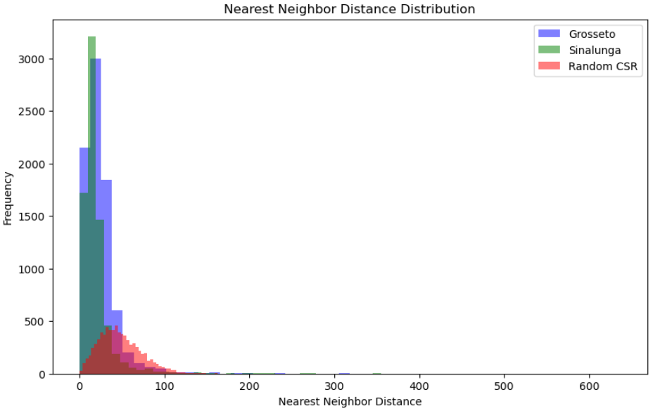
The values for the second city are more clustered.
Mean nearest neighbor distance for observed points in the first city: 24.73
Mean nearest neighbor distance for observed points in the second city: 19.96

3.2 Comparing two Cities

The code compares the mean nearest neighbor distances between the first city and the second city. If the mean distance for the second city is less than that of the first city, indicating greater clustering, a message is printed to convey this observation along with the respective mean distances for both cities. Conversely, if the mean distance for the second city is greater, suggesting more dispersion, another message is printed with the corresponding mean distances for both cities. The results suggest that the buildings of Sinalunga are more clustered than the ones in Grosseto.

# Plot histograms of nearest neighbor distances
plt.figure(figsize=(10, 6))
plt.hist(nearest_neighbor_distances(coordinates), bins=50, color='blue', alpha=0.5, label='Grosseto')
plt.hist(nearest_neighbor_distances(coordinates2), bins=50, color='green', alpha=0.5, label='Sinalunga')
plt.hist(nearest_neighbor_distances(coordinates_random), bins=50, color='red', alpha=0.5, label='Random CSR')
plt.xlabel('Nearest Neighbor Distance')
plt.ylabel('Frequency')
plt.title('Nearest Neighbor Distance Distribution')
plt.legend()
plt.show()

Finally, we can display an histogram comparing the random distribution with the NDD values of each point for Grosseto and Sinalunga. Overall, this approach can be useful for various analytical purposes, such as comparing whether a subset of data is more or less clustered than the main dataset (e.g., a subset containing missing values) or for examining specific typologies within a dataset. It could also be interesting to compare the results of a single city at different periods. A lower score between two periods would suggest a densification process, whereas a larger score would indicate a dynamic of urban sprawl.

References & to go further

• Point Pattern Analysis – Geographic Data Science
• Yuan, Y., Qiang, Y., Bin Asad, K., and Chow, T. E. (2020). Point Pattern Analysis. The Geographic Information Science & Technology Body of Knowledge (1st Quarter 2020 Edition), John P. Wilson (ed.). DOI: 10.22224/gistbok/2020.1.13.
• Usui, H and Perez, J. (2020) “Are patterns of vacant lots random? Evidence from empirical spatiotemporal analysis in Chiba prefecture, east of Tokyo”, Environment and Planning B: Urban Analytics and City Science, 49(3). Read more